Automata¶

Two main classes of automata are implemented: Labelled Transition Systems and Finite Automata.

Labelled Transition Systems¶

Labelled transition systems are created using the libmc.LTS class:

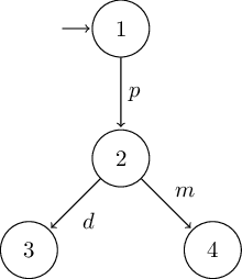
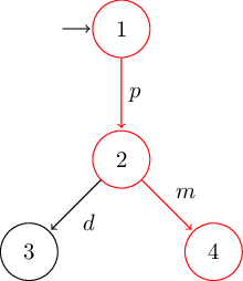
# deterministic version of Milner's vending machine
G = LTS(
    S = [1, 2, 3, 4],
    I = [1],
    Σ = ['p', 'd', 'm'],
    T = [
            (1, 'p', 2),
            (2, 'd', 3),
            (2, 'm', 4),
        ]
)

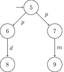
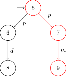
# nondeterministic version of Milner's vending machine
B = LTS(
    S = [5, 6, 7, 8, 9],
    I = [5],
    Σ = ['p', 'd', 'm'],
    T = [
            (5, 'p', 6),
            (5, 'p', 7),
            (6, 'd', 8),
            (7, 'm', 9),
        ]
)

Note

Due to limitations of sets in python (hashability), automata components are lists instead of sets.

Finite Automata¶

Finite automata are created using the libmc.FA class:

# (un)?sat
F = FA(
    S = [1, 2, 3, 4, 5, 6],
    I = [1],
    Σ = ['u', 'n', 's', 'a', 't'],
    T = [
            (1, 's', 4),
            (1, 'u', 2),
            (2, 'n', 3),
            (3, 's', 4),
            (4, 'a', 5),
            (5, 't', 6)
        ],
    F = [6]
)

Note

As a subclass of libmc.LTS they support the same methods and more.

Acceptance¶

libmc.FA supports testing the acceptance of a given word using the accepts() method:

assert F.accepts("sat")
assert F.accepts("unsat")
assert not F.accepts("santa")

Completeness and Determinism¶

Completeness as well as determinism can be checked using isComplete() and isDeterministic() respectively:

assert not G.isComplete()
assert not B.isComplete()

assert G.isDeterministic()
assert not B.isDeterministic()

Product¶

Product automata are created with the product() method:

GB = G.product(B)

assert GB.S == [(1, 5), (2, 6), (2, 7), (3, 8), (4, 9)]
assert GB.I == [(1, 5)]
assert GB.Σ == ['p', 'd', 'm']
assert GB.T == [
    ((1, 5), 'p', (2, 6)),
    ((1, 5), 'p', (2, 7)),
    ((2, 6), 'd', (3, 8)),
    ((2, 7), 'm', (4, 9))
]

Sub-Set Construction¶

Power automata are created with the power() method:

P = B.power()

assert P.isComplete()
assert P.isDeterministic()

assert P.S == [[], [5], [6, 7], [8], [9]]
assert P.I == [[5]]
assert P.Σ == B.Σ
assert P.T == [
    ([], 'd', []),
    ([], 'm', []),
    ([], 'p', []),
    ([5], 'd', []),
    ([5], 'm', []),
    ([5], 'p', [6, 7]),
    ([6, 7], 'd', [8]),
    ([6, 7], 'm', [9]),
    ([6, 7], 'p', []),
    ([8], 'd', []),
    ([8], 'm', []),
    ([8], 'p', []),
    ([9], 'd', []),
    ([9], 'm', []),
    ([9], 'p', [])
]

Complement¶

The complement of a libmc.FA is created with the complement() method:

C = F.complement()

assert C.S == F.S
assert C.I == F.I
assert C.Σ == F.Σ
assert C.T == F.T
assert C.F == [1, 2, 3, 4, 5]

Traces¶

The trace() method offers a way to find all paths (list of transitions) from one state to another:

# find the milky way
traces = G.trace(4)

assert traces == [[(1, 'p', 2), (2, 'm', 4)]]

Conformance¶

Checking the conformance of one libmc.FA to another is carried out with the conforms() method:

# automaton modelling the implementation
I = FA(
    S = ['1', '2', '3', '4'],
    I = ['1'],
    Σ = Σ,
    T = [
            ('1', 'b', '2'),
            ('2', 'b', '3'),
            ('2', 'b', '4'),
            ('3', 'a', '1'),
            ('3', 'b', '3'),
            ('4', 'b', '3')
        ],
    F = ['4']
)

# automaton modelling the specification
S = FA(
    S = ['A', 'B', 'C', 'D'],
    I = ['A'],
    Σ = Σ,
    T = [
            ('A', 'a', 'C'),
            ('A', 'a', 'D'),
            ('A', 'b', 'A'),
            ('A', 'b', 'B'),
            ('B', 'a', 'D'),
            ('B', 'b', 'C'),
            ('C', 'a', 'C'),
            ('C', 'a', 'D'),
            ('D', 'b', 'A')
        ],
    F = ['B']
)

conforms, ICPS, traces = I.conforms(S)

assert conforms
assert not traces

Simulation¶

simulates() can be used to check if a libmc.LTS simulates another:

# G simulates B?
simulates = G.simulates(B)
simulation = maximumSimulation(B, G, set(product(B.S, G.S)))

assert simulates
assert simulation == {
    (5, 1),
            (6, 2),
            (7, 2),
    (8, 1), (8, 2), (8, 3), (8, 4),
    (9, 1), (9, 2), (9, 3), (9, 4)
}

# B simulates G?
simulates = B.simulates(G)
simulation = maximumSimulation(G, B, set(product(G.S, B.S)))

assert not simulates
assert simulation == {
    (3, 5), (3, 6), (3, 7), (3, 8), (3, 9),
    (4, 5), (4, 6), (4, 7), (4, 8), (4, 9)
}

To just generate the simulation relation, use libmc.maximumSimulation():

# full simulation relation
simulation = \
    maximumSimulation(G, G, set(product(G.S, G.S))) | \
    maximumSimulation(G, B, set(product(G.S, B.S))) | \
    maximumSimulation(B, G, set(product(B.S, G.S))) | \
    maximumSimulation(B, B, set(product(B.S, B.S)))

assert simulation == {
    (1, 1),
            (2, 2),
    (3, 1), (3, 2), (3, 3), (3, 4), (3, 5), (3, 6), (3, 7), (3, 8), (3, 9),
    (4, 1), (4, 2), (4, 3), (4, 4), (4, 5), (4, 6), (4, 7), (4, 8), (4, 9),
    (5, 1),                         (5, 5),
            (6, 2),                         (6, 6),
            (7, 2),                                 (7, 7),
    (8, 1), (8, 2), (8, 3), (8, 4), (8, 5), (8, 6), (8, 7), (8, 8), (8, 9),
    (9, 1), (9, 2), (9, 3), (9, 4), (9, 5), (9, 6), (9, 7), (9, 8), (9, 9)
}

Weak Simulation¶

In order to perform a weak simulation, add the set of internal events τ:

A1 = LTS(
    S = [1, 2, 3],
    I = [1],
    Σ = ['a', 'b', 'τ'],
    T = [
            (1, 'b', 3),
            (1, 'τ', 2),
            (2, 'a', 3),
            (3, 'τ', 1)
        ]
)

A2 = LTS(
    S = [4, 5],
    I = [4],
    Σ = ['a', 'b', 'τ'],
    T = [
            (4, 'a', 4),
            (4, 'b', 5),
            (5, 'a', 4),
            (5, 'τ', 4)
        ]
)

# internal events
τ = ['τ']

# full simulation relation
simulation = \
    maximumSimulation(A1, A1, set(product(A1.S, A1.S)), τ) | \
    maximumSimulation(A1, A2, set(product(A1.S, A2.S)), τ) | \
    maximumSimulation(A2, A1, set(product(A2.S, A1.S)), τ) | \
    maximumSimulation(A2, A2, set(product(A2.S, A2.S)), τ)

assert simulation == {
    (1, 1),         (1, 3), (1, 4), (1, 5),
    (2, 1), (2, 2), (2, 3), (2, 4), (2, 5),
    (3, 1),         (3, 3), (3, 4), (3, 5),
    (4, 1),         (4, 3), (4, 4), (4, 5),
    (5, 1),         (5, 3), (5, 4), (5, 5)
}

# A1 simulates A2?
simulates = A1.simulates(A2, τ)
simulation = maximumSimulation(A2, A1, set(product(A2.S, A1.S)), τ)

assert simulates
assert simulation == {(4, 1), (4, 3), (5, 1), (5, 3)}

# A2 simulates A1?
simulates = A2.simulates(A1, τ)
simulation = maximumSimulation(A1, A2, set(product(A1.S, A2.S)), τ)

assert simulates
assert simulation == {(1, 4), (1, 5), (2, 4), (2, 5), (3, 4), (3, 5)}

Bisimulation¶

Bisimulations are tested in a similar manner by using bisimulates() and libmc.maximumBisimulation():

# G bisimulates B?
simulates = G.bisimulates(B)

# full simulation relation
simulation = \
    maximumBisimulation(G, G, set(product(G.S, G.S))) | \
    maximumBisimulation(G, B, set(product(G.S, B.S))) | \
    maximumBisimulation(B, G, set(product(B.S, G.S))) | \
    maximumBisimulation(B, B, set(product(B.S, B.S)))

assert not simulates
assert simulation == {
    (1, 1),
            (2, 2),
                    (3, 3), (3, 4),                         (3, 8), (3, 9),
                    (4, 3), (4, 4),                         (4, 8), (4, 9),
                                    (5, 5),
                                            (6, 6),
                                                    (7, 7),
                    (8, 3), (8, 4),                         (8, 8), (8, 9),
                    (9, 3), (9, 4),                         (9, 8), (9, 9)
}

Minimization¶

Minimize a deterministic libmc.FA with minimize():

F = FA (
    S = ['A', 'B', 'C', 'D', 'E', 'F'],
    I = ['A'],
    Σ = [0, 1],
    T = [
            ('A', 0, 'B'),
            ('A', 1, 'E'),
            ('B', 0, 'A'),
            ('B', 1, 'C'),
            ('C', 0, 'A'),
            ('C', 1, 'C'),
            ('D', 0, 'F'),
            ('D', 1, 'C'),
            ('E', 0, 'D'),
            ('E', 1, 'E'),
            ('F', 0, 'A'),
            ('F', 1, 'E')
        ],
    F = ['B', 'F']
)

assert F.isDeterministic()

minF = F.minimize()

assert minF.S == [('A', 'D'), ('B', 'F'), ('C', 'E')]
assert minF.I == [('A', 'D')]
assert minF.Σ == F.Σ
assert minF.T == [
    (('A', 'D'), 0, ('B', 'F')),
    (('A', 'D'), 1, ('C', 'E')),
    (('B', 'F'), 0, ('A', 'D')),
    (('B', 'F'), 1, ('C', 'E')),
    (('C', 'E'), 0, ('A', 'D')),
    (('C', 'E'), 1, ('C', 'E'))
]
assert minF.F == [('B', 'F')]

Asynchronous Composition¶

Generate the automaton modelling the asynchronous composition of two or more libmc.LTS with libmc.asynchronousComposition():

A1 = LTS(
    S = [1, 2, 3, 4],
    I = [1],
    Σ = ['a', 'b', 'c', 's'],
    T = [
            (1, 'a', 2),
            (2, 'b', 3),
            (3, 'c', 4),
            (4, 's', 1)
        ]
    )

A2 = LTS(
    S = [5, 6, 7, 8],
    I = [5],
    Σ = ['d', 'e', 'f', 's'],
    T = [
            (5, 'd', 6),
            (6, 'e', 7),
            (7, 'f', 8),
            (8, 's', 5),
        ]
    )

composition = asynchronousComposition(A1, A2)

assert composition.S == [
    (1, 5), (1, 6), (1, 7), (1, 8),
    (2, 5), (2, 6), (2, 7), (2, 8),
    (3, 5), (3, 6), (3, 7), (3, 8),
    (4, 5), (4, 6), (4, 7), (4, 8)
]
assert composition.I == [(1, 5)]
assert composition.Σ == ['a', 'b', 'c', 'd', 'e', 'f', 's']
assert composition.T == [
    ((1, 5), 'a', (2, 5)), ((1, 5), 'd', (1, 6)),
    ((1, 6), 'a', (2, 6)), ((1, 6), 'e', (1, 7)),
    ((1, 7), 'a', (2, 7)), ((1, 7), 'f', (1, 8)),
    ((1, 8), 'a', (2, 8)), ((2, 5), 'b', (3, 5)),
    ((2, 5), 'd', (2, 6)), ((2, 6), 'b', (3, 6)),
    ((2, 6), 'e', (2, 7)), ((2, 7), 'b', (3, 7)),
    ((2, 7), 'f', (2, 8)), ((2, 8), 'b', (3, 8)),
    ((3, 5), 'c', (4, 5)), ((3, 5), 'd', (3, 6)),
    ((3, 6), 'c', (4, 6)), ((3, 6), 'e', (3, 7)),
    ((3, 7), 'c', (4, 7)), ((3, 7), 'f', (3, 8)),
    ((3, 8), 'c', (4, 8)), ((4, 5), 'd', (4, 6)),
    ((4, 6), 'e', (4, 7)), ((4, 7), 'f', (4, 8)),
    ((4, 8), 's', (1, 5))
]

Partial Order Reduction¶

Perform partial order reduction by supplying a function choosing the index of the components used for local expansion:

# with partial order reduction, expanding the rightmost component
composition = asynchronousComposition(A1, A2, partialOrderReduction = lambda x: [x[-1]])

assert composition.S == [(1, 5), (1, 6), (1, 7), (1, 8), (2, 8), (3, 8), (4, 8)]
assert composition.I == [(1, 5)]
assert composition.Σ == ['a', 'b', 'c', 'd', 'e', 'f', 's']
assert composition.T == [
    ((1, 5), 'd', (1, 6)),
    ((1, 6), 'e', (1, 7)),
    ((1, 7), 'f', (1, 8)),
    ((1, 8), 'a', (2, 8)),
    ((2, 8), 'b', (3, 8)),
    ((3, 8), 'c', (4, 8)),
    ((4, 8), 's', (1, 5))
]

Visualization¶

Last but not least, automata may be visualized in two ways: either using the DOT language or as a customizable TikZ based LaTeX figure.

DOT¶

toDot() offers an easy way to generate a graphical representation of the given automaton using Graphviz in combination with dot2tex:

dot = G.toDot()
with open("/tmp/milner-deterministic-toDot.dot", 'w') as f:
    f.write(dot)

dot = B.toDot()
with open("/tmp/milner-nondeterministic-toDot.dot", 'w') as f:
    f.write(dot)

After generating the DOT language string, use dot2tex to convert it into a TikZ based LaTeX figure:

$ dot2tex --template=dot2tex-template.tex /tmp/milner-deterministic-toDot.dot > /tmp/milner-deterministic-toDot.tex
$ dot2tex --template=dot2tex-template.tex /tmp/milner-nondeterministic-toDot.dot > /tmp/milner-nondeterministic-toDot.tex

Using this minimal dot2tex latex template results in the following graphs:

_images/milner-nondeterministic-toDot.png

TikZ¶

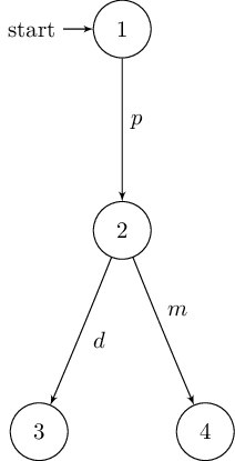
toTex() generates a customizable TikZ based LaTeX figure (tikzpicture):

tex = G.toTex()
with open("/tmp/milner-deterministic-toTex.tex", 'w') as f:
    f.write(tex)

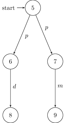
tex = B.toTex()
with open("/tmp/milner-nondeterministic-toTex.tex", 'w') as f:
    f.write(tex)

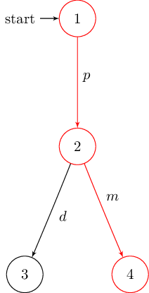
In case of the deterministic version of Milner’s vending machine it returns:

% requires following LaTex preamble:
% \usepackage{tikz}
% \usetikzlibrary{arrows,automata}
\begin{tikzpicture}[shorten >=1pt,node distance=2cm,auto,initial text=]

  % manual positioning required!
  \node[state,initial]          (1)                          {$1$};
  \node[state]                  (2)                          {$2$};
  \node[state]                  (3)                          {$3$};
  \node[state]                  (4)                          {$4$};

  \path[->]          (1)   edge                node          {$p$} (2);
  \path[->]          (2)   edge                node          {$d$} (3);
  \path[->]          (2)   edge                node          {$m$} (4);
\end{tikzpicture}

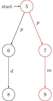
Since no automatic layouting is performed, nodes need to be placed manually. This might be beneficial if the DOT file’s layout is suboptimal. To do so, just add the usual TikZ directives:

% requires following LaTex preamble:
% \usepackage{tikz}
% \usetikzlibrary{arrows,automata}
\begin{tikzpicture}[shorten >=1pt,node distance=2cm,auto,initial text=]

  % manual positioning required!
  \node[state,initial]          (1)                          {$1$};
  \node[state]                  (2) [below of=1]             {$2$};
  \node[state]                  (3) [below left of=2]        {$3$};
  \node[state]                  (4) [below right of=2]       {$4$};

  \path[->]          (1)   edge                node          {$p$} (2);
  \path[->]          (2)   edge                node          {$d$} (3);
  \path[->]          (2)   edge                node          {$m$} (4);
\end{tikzpicture}